Pulseq in.
Realistic raw data out.
BlochTwin is an MRI simulator for research. It runs your pulse sequence on a head phantom built from real human data and returns what a scanner would have recorded: multi-coil k-space with correlated receiver noise, the reconstructed images, and the ground truth behind them.
Working at a company? Ask about an evaluation.
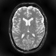
From a sequence file to raw data
1.Give it a sequence
Upload a Pulseq file. Every RF pulse, gradient and ADC event is simulated as written, so a new sequence needs no new code on our side.
Or start from a built-in gradient echo, spin echo, turbo spin echo, FLAIR or EPI and set its parameters.
Figure 2a. The sequence behind Figure 1 as the engine read it from the Pulseq file: the excitation, the first five of the 20 refocusing pulses and four readouts, the first 46 ms of a 4 s repetition. The whole file has 1,804 blocks. 2.Choose the head and the scanner
The phantom stores how much of each tissue every voxel holds, so a voxel on a boundary is a mixture, as in a real head. At the field strength you choose (1.5, 3 or 7 T) each tissue takes its T1, T2 and T2* from literature tables. At 3 T, the default, the deep nuclei’s T1 comes from measured T1 maps of 16 adults.
The susceptibility field, the transmit field and the receive array are computed for that same head.
0.32.6 sT1 −60+60 HzΔB0 after shim
 0.801.25B1+
 receive sensitivity4 of 32 loops
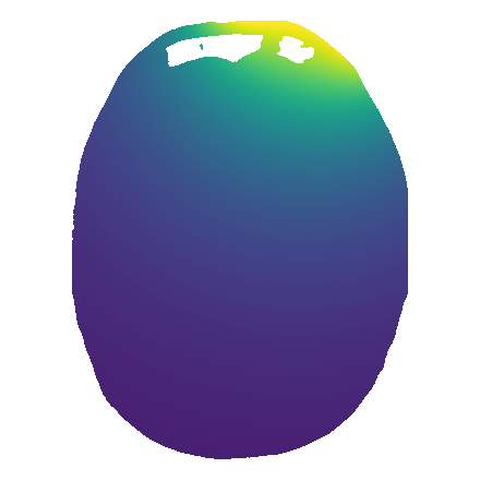
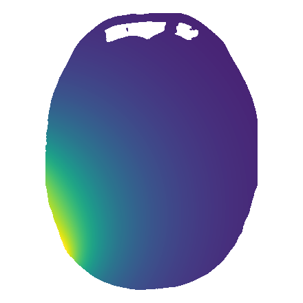
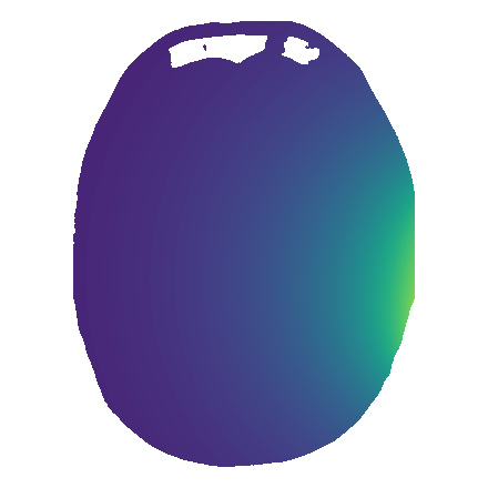
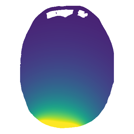
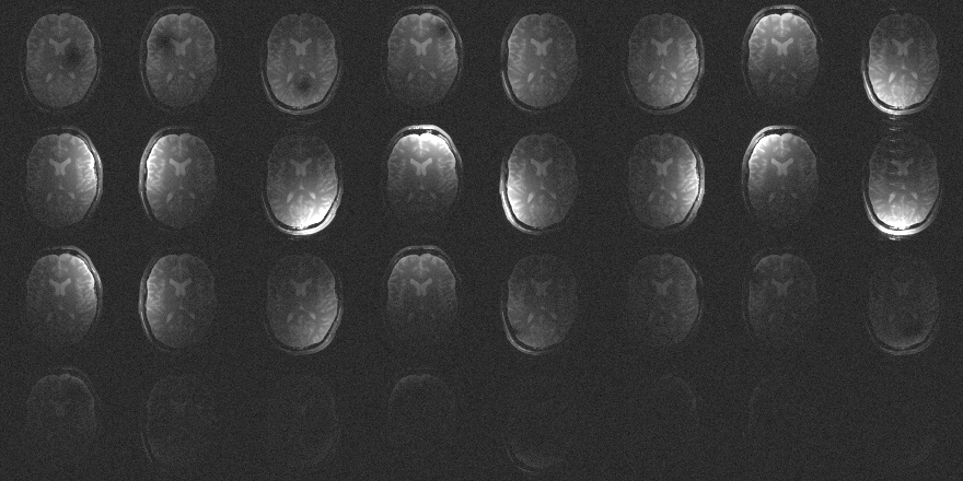
Figure 2b. What the simulation is given for the slice of Figure 1, at 3 T: the phantom’s T1, the field offset left after second-order shimming (the dipole pattern in front comes from the air of the frontal sinus), the transmit field, and the sensitivity of four of the receive loops. 3.Download what the receiver recorded, and what it could not
The raw data arrive in the format your reconstruction already reads. Beside them comes everything the simulation knew and a scanner never does: the answer your method is trying to recover.
You get Format As from a scanner Raw k-space, every channel, with a noise scan ISMRMRD Reconstructed images NIfTI, PNG Only from a simulation The same raw data without noise ISMRMRD The receive sensitivities the simulation used NIfTI Tissue fractions and parameter maps NIfTI The head pose at every k-space line, if it moved JSON The predicted sound of the gradients WAV Run record: engine version, seed, every parameter JSON
The same three steps from Python, for a parameter sweep or a notebook. Submitting and viewing in the browser work without it.
import blochtwin as bt

run = bt.simulate(
    sequence="my_tse.seq",    # any 2D Pulseq file
    phantom="head-1mm",
    field_strength=3.0,       # tesla
    coils=32,
    noise=True,
    seed=7,
)
run.download("raw.h5")        # ISMRMRD, 32 channels, noise scan included
truth = run.noise_free_kspace()Look at the output before you sign up
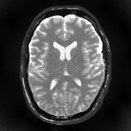
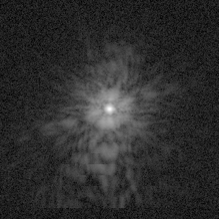
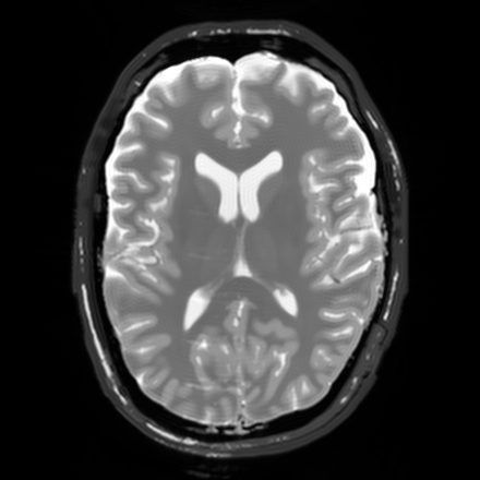
Seven scans of one slice, computed by the engine and shown as they came out. Pick one and read its k-space next to it.
Cerebrospinal fluid bright, the echo train's T2 decay in k-space.
- TR / TE
- 4000 / 96 ms
- Echo train
- 20 echoes, 9.6 ms apart
- Matrix
- 220 × 220 over 220 mm
- Scan time
- 0:44
- Field
- 3 T
- Receive
- 32 channels
- Slice
- axial, 4 mm
What is in the signal
Each effect enters where it does in a scanner: in the magnetisation, in the field or in the receive chain. All of them are available on every plan.
Magnetisation
- Bloch simulation of any Pulseq sequence: RF pulses as rotations in 10 µs steps, exact precession and relaxation in between (Bloch 1946; Pauly 1991; Layton 2017).
- Slice profiles that follow from the RF waveform and its gradient, and cross-talk between neighbouring slices.
- Reversible dephasing inside a voxel (T2′): gradient echoes decay with T2*, spin echoes refocus it (Endres 2024).
- Tissue values at 1.5, 3 and 7 T from literature tables (Rooney 2007); at 3 T the deep nuclei’s T1 from MP2RAGE maps of 16 adults, and T2* of white matter, cortex and deep nuclei from a 12-echo gradient echo of 18 adults (OpenNeuro ds004958). The variation inside each tissue is taken from the person the phantom was built from.
- Fat with a six-peak spectrum, so chemical shift and its dephasing appear on their own (Yu 2008).
Fields and the subject
- ΔB0 from the head’s own susceptibility, air cavities included, after centre-frequency and second-order shim (Salomir 2003; Marques 2005).
- A transmit-field map with the central brightening of a head at 3 T (a smooth model, not a field calculation).
- Rigid head motion during the scan, line by line in k-space (Zaitsev 2015).
- Breathing as a field fluctuation; blood that pulses with the heartbeat, with its inflow enhancement and wash-out.
- The sound of the sequence, from its gradient waveforms through a transfer model built on published measurements of gradient coils (Hedeen 1997).
Receive chain
- Array sensitivities from the fields of the loops, by reciprocity; 1, 8 or 32 channels on a helmet (Hoult 1976).
- Thermal noise added to k-space per channel, correlated between channels through the conducting head (Roemer 1990). Rician statistics in magnitude images follow from it (Gudbjartsson 1995).
- A noise scan in front of the data, as a scanner records it.
- Reconstruction you can replace: root-sum-of-squares with prescan normalisation or noise prewhitening, SENSE (Pruessmann 1999), partial Fourier.
Not modelled yet. Gradient delays and eddy currents, concomitant fields, coupling between receive coils, RF wavelength effects at 7 T, diffusion and magnetisation transfer. Head motion, breathing and pulsing blood work with the built-in sequences today and not yet with an uploaded Pulseq file. A whole-head 3D scan takes hours to simulate at 2 mm and far longer below it, which is why the free plan starts with 2D.
Checked against closed forms, another simulator and a scanner
The source is closed, so the evidence has to be open. The band for a pass was fixed before the measured data were looked at, and what falls outside it stays in the table.
| Compared | Against | Result | Verdict |
|---|---|---|---|
| Spin echo, inversion recovery and flip-angle signals of single voxels | Closed-form solutions of the Bloch equations | Identical to machine precision | agrees |
| The same experiments, white matter, grey matter and CSF | KomaMRI (Castillo-Passi 2023) | Mean absolute difference 0.0023 %, worst 0.0113 % | agrees |
| Dephasing inside a voxel across a spin-echo readout | exp(−t/T2) exp(−R2′|t − TE|) | Within 0.2 %, cusp included | agrees |
| Receiver noise after prewhitening | The covariance that was put in | Channel correlation below 0.02; covariance recovered within 2 % | agrees |
| Noise correlation between the channels of a 32-channel head array | Noise scan of a 7 T head coil (Lüsebrink 2021) | Measured mean |ρ| 0.06; model 0.12 to 0.25 | too high, 2 to 4 times |
| MPRAGE at 7 T, same person: white-matter signal, 5° scan over 1° scan | The scanner’s images | Measured 5.09, predicted 5.02 | agrees |
| Same scans: where the boundary between grey and white matter lies, and how sharp it is | The scanner’s images | Position within 0.02 mm, width 0.47 against 0.46 mm | agrees |
| Same scans: contrast to white matter, predicted over measured. Pass band 0.9 to 1.1 | The scanner’s images | Cortical grey matter 0.93 | inside the band |
| Caudate 0.89 | just outside | ||
| Putamen 0.82, thalamus 0.75, pallidum 0.73, CSF 1.43 | outside the band |
Where it does not match
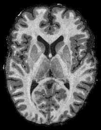
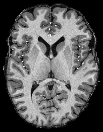
Deep nuclei. Caudate, putamen, thalamus and pallidum are all brighter in the scan than predicted: in this person their T1 is 5 to 19 % shorter than the literature table. The phantom carries each tissue’s variation, not yet this person’s own tissue means.
Cortex. Measured grey matter is brighter next to white matter than at the outer surface (0.62 falling to 0.54 of white matter); the prediction is nearly flat at 0.52 to 0.54. The phantom has one T1 through the depth of the cortex.
Transmit field. The comparison assumes it uniform. At 7 T it is not, and these scans cannot tell us what it was.
Outside the brain. Scalp, face and neck were left out: the shading correction is fitted to white matter and does not hold there.
What it is for
Trying a sequence before the scanner is free
Contrast, slice profile, what off-resonance and motion do to it, and how loud it will be: from the file you would take to the scanner.
Testing reconstruction and learning methods
Multi-coil raw data with the noise-free k-space, the sensitivities and the tissue maps they came from. Change one factor at a time (noise, motion, field strength) and score against the truth.
Checking a quantitative method
The T1, T2 and proton density of every voxel are known, so a mapping sequence and its fit can be compared with the values that went in.
Free for academic research in 2D
The plans differ in dimensions, phantoms, compute and what you may do with the results. The physics is the same on all of them. The free plan opens first.
| Property | Community | Researcher and Lab | Industry |
|---|---|---|---|
| For | Researchers at universities, institutes and hospitals | The same, when 2D is not enough | Companies |
| Price | Free | To be announced | By contract, after an evaluation |
| Dimensions | 2D, multi-slice included | 2D and 3D | 2D and 3D |
| Phantoms | Shepp–Logan, vial phantom, procedural head, a real head at 1 mm | Adds the 0.5 mm head, lesions and, for a lab, your own phantoms | Adds phantoms built to order |
| Physics options | All | All | All |
| Compute | A monthly allowance; the cost of a run is shown before it starts | A larger allowance, several runs at once | By contract |
| Ways in | Browser, API, Python client | Adds batch submission | Adds dataset generation |
| Use of results | Non-commercial research, with a citation | The same | Commercial use, training data included |
| Opens | First, to invited groups, then to everyone | After the free plan | Evaluation by approval, seven days |
Questions
The source is closed. Why should I trust the output?
Because you can check it without reading our code. Sequences go in as Pulseq files and data come out as ISMRMRD and NIfTI, so you can reconstruct the raw data with your own tools and set it beside your own scans. The physics is documented with its sources, and the table above lists every check, the failed ones included. Each result records the engine version, the random seed and every parameter.
What happens to a sequence I upload?
It stays yours. We use it to run your simulation and for nothing else, and we delete it when you ask. The terms of use will say so in full before sign-up opens.
How do I cite it?
Every result comes with a citation line and its run record. A technical report on the engine and its validation is in preparation; cite that once it is out.
Will the same run give the same numbers next year?
A result belongs to an engine version. Older versions stay available for re-running for a fixed period, which the terms of use will state.
Who counts as academic?
Anyone doing non-commercial research at a university, a research institute or a hospital who signs in with that institution’s email address. An address we cannot recognise automatically is looked at by a person.
Can a company use it?
Yes, on the Industry plan. An evaluation runs for seven days once it is approved. Results from an evaluation or from an academic plan may not be used commercially.
Is it a medical device?
No. BlochTwin is a research tool. Its output must not be used for diagnosis or for decisions about treatment.
Request access with your institutional email
For a company evaluation or anything else, write to contact@newmean.ai.
References
- Bloch F. Nuclear induction. Phys Rev 70, 460–474 (1946).
- Castillo-Passi C, et al. KomaMRI.jl: an open-source framework for general MRI simulations with GPU acceleration. Magn Reson Med 90, 329–342 (2023).
- Endres J, et al. Phase distribution graphs for fast, differentiable, and spatially encoded Bloch simulations of arbitrary MRI sequences. Magn Reson Med 92, 1189–1204 (2024).
- Gudbjartsson H, Patz S. The Rician distribution of noisy MRI data. Magn Reson Med 34, 910–914 (1995).
- Hedeen RA, Edelstein WA. Characterization and prediction of gradient acoustic noise in MR imagers. Magn Reson Med 37, 7–10 (1997).
- Hoult DI, Richards RE. The signal-to-noise ratio of the nuclear magnetic resonance experiment. J Magn Reson 24, 71–85 (1976).
- Layton KJ, et al. Pulseq: a rapid and hardware-independent pulse sequence prototyping framework. Magn Reson Med 77, 1544–1552 (2017).
- Lüsebrink F, et al. Comprehensive ultrahigh resolution whole brain in vivo MRI dataset as a human phantom. Sci Data 8, 138 (2021). OpenNeuro ds003563.
- Marques JP, Bowtell R. Application of a Fourier-based method for rapid calculation of field inhomogeneity due to spatial variation of magnetic susceptibility. Concepts Magn Reson B 25B, 65–78 (2005).
- Pauly J, et al. Parameter relations for the Shinnar–Le Roux selective excitation pulse design algorithm. IEEE Trans Med Imaging 10, 53–65 (1991).
- Pruessmann KP, et al. SENSE: sensitivity encoding for fast MRI. Magn Reson Med 42, 952–962 (1999).
- Roemer PB, et al. The NMR phased array. Magn Reson Med 16, 192–225 (1990).
- Rooney WD, et al. Magnetic field and tissue dependencies of human brain longitudinal 1H2O relaxation in vivo. Magn Reson Med 57, 308–318 (2007).
- Salomir R, et al. A fast calculation method for magnetic field inhomogeneity due to an arbitrary distribution of bulk susceptibility. Concepts Magn Reson B 19B, 26–34 (2003).
- Yu H, et al. Multiecho water-fat separation and simultaneous R2* estimation with multifrequency fat spectrum modeling. Magn Reson Med 60, 1122–1134 (2008).
- Zaitsev M, et al. Motion artifacts in MRI: a complex problem with many partial solutions. J Magn Reson Imaging 42, 887–901 (2015).